Predator prey
This page contains a description predator prey model that is used as a running example throughout the text. A detailed description of the dynamics of this system is presented in Chapter 3 - Examples and these dynamics are analyzed in Chapter 4 - Dynamic Behavior. A state space feedback controller is designed in Chapter 6 - State Feedback. This page brings together this material into a single place, to illustrate the application of analysis and design tools for this system. Links to MATLAB scripts are included that generate the analysis and figures described here.
System Description
The predator-prey problem refers to an ecological system in which we have two species, one of which feeds on the other. This type of system has been studied for decades and is known to exhibit interesting dynamics. The figure below shows a historical record taken over 90 years for a population of lynxes versus a population of hares (MacLulich, 1937).

|

|
|||
|
Figure 2.6: Predator versus prey. The photograph on the left shows a Canadian lynx and a snowshoe hare, the lynx’s primary prey. The graph on the right shows the populations of hares and lynxes between 1845 and 1935 in a section of the Canadian Rockies (MacLuluch, 1937). The data were collected on an annual basis over a period of 90 years. (Photograph copyright Tom and Pat Leeson.) | ||||
Discrete Time Model
A simple model for this situation can be constructed using a discrete-time
model by keeping track of the rate of births and deaths of each species.
Letting  represent the population of hares and
  represent the
population of lynxes, we can describe the state in terms of the
populations at discrete periods of time. Letting
represent the
population of lynxes, we can describe the state in terms of the
populations at discrete periods of time. Letting  be the
discrete-time index (e.g., the day or month number), we can write
be the
discrete-time index (e.g., the day or month number), we can write
|
|
(2.13) |
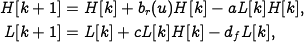
where  is the hare birth rate per unit period and as a
function of the food supply
is the hare birth rate per unit period and as a
function of the food supply  ,
,  is the lynx mortality rate and
  and
and  are the interaction coefficients.
The interaction term
are the interaction coefficients.
The interaction term  models
the rate of predation, which is assumed to be proportional to the rate
at which predators and prey meet and is hence given by the product of
the population sizes. The interaction term
models
the rate of predation, which is assumed to be proportional to the rate
at which predators and prey meet and is hence given by the product of
the population sizes. The interaction term  in the
lynx dynamics has a similar form and represents the rate of growth of
the lynx population. This model makes many simplifying
assumptions -- such as the fact that hares decrease in number only
through predation by lynxes -- but it often is sufficient to answer
basic questions about the system.
in the
lynx dynamics has a similar form and represents the rate of growth of
the lynx population. This model makes many simplifying
assumptions -- such as the fact that hares decrease in number only
through predation by lynxes -- but it often is sufficient to answer
basic questions about the system.
To illustrate the use of this system, we can compute the number of lynxes
and hares at each time point from some initial population. This is
done by starting with 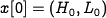 and then using equation (2.13) to compute
the populations in the following period. By iterating this procedure, we can
generate the population over time. The output of this process for a specific
choice of parameters and initial conditions is shown below:
and then using equation (2.13) to compute
the populations in the following period. By iterating this procedure, we can
generate the population over time. The output of this process for a specific
choice of parameters and initial conditions is shown below:

Using the parameters  ,
,
 and
and  in
equation~\eqref{eq:modeling:predprey} with daily updates, the
period and magnitude of the lynx and hare population cycles
approximately match the data in Figure 2.4. While the details of
the simulation are different from the experimental data (to be
expected given the simplicity of our assumptions), we see
qualitatively similar trends and hence we can use the model to
help explore the dynamics of the system.
in
equation~\eqref{eq:modeling:predprey} with daily updates, the
period and magnitude of the lynx and hare population cycles
approximately match the data in Figure 2.4. While the details of
the simulation are different from the experimental data (to be
expected given the simplicity of our assumptions), we see
qualitatively similar trends and hence we can use the model to
help explore the dynamics of the system.
MATLAB files for the discrete time model:
- predprey_discrete.m - discrete time simulation of predator prey model
Continuous Time Model
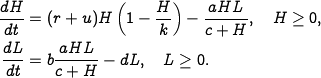
We now replace the difference equation model
used there with a more sophisticated differential equation model. Let  represent the number of hares (prey) and let
  represent the number of
lynxes (predator). The dynamics of the system are modeled as
represent the number of
lynxes (predator). The dynamics of the system are modeled as
|
|
(3.31) |
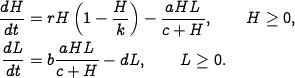
In the first equation,  represents the growth rate of the hares,
represents the maximum population of the hares (in the absence of
lynxes),\index{carrying capacity, in population models} represents
the interaction term that describes how the
hares are diminished as a function of the lynx population and
controls the prey consumption rate for low hare population. In the
second equation,
represents the growth rate of the hares,
represents the maximum population of the hares (in the absence of
lynxes),\index{carrying capacity, in population models} represents
the interaction term that describes how the
hares are diminished as a function of the lynx population and
controls the prey consumption rate for low hare population. In the
second equation,  represents the growth coefficient of the lynxes
and
represents the growth coefficient of the lynxes
and  represents the mortality rate of the lynxes.
Note that the hare dynamics include a term that resembles the
logistic growth model (3.30) in Chapter 3 - Examples.
represents the mortality rate of the lynxes.
Note that the hare dynamics include a term that resembles the
logistic growth model (3.30) in Chapter 3 - Examples.
Of particular interest are the values at which the population values
remain constant, called equilibrium points.
The equilibrium points for this system can be determined by setting
the right-hand side of the above equations to zero. Letting  and
and
 represent the equilibrium state, from the second equation we
have
represent the equilibrium state, from the second equation we
have
|
|
(3.32) |
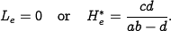
Substituting this into the first equation, we have that for  either
  or
or  . For
. For  , we obtain
|
|
(3.33) |
Thus, we have three possible equilibrium points  :
:
where  and
and  are given in
equations (3.32)
and (3.33). Note that the equilibrium
populations may be negative for some parameter values, corresponding to a
nonachievable equilibrium point.
are given in
equations (3.32)
and (3.33). Note that the equilibrium
populations may be negative for some parameter values, corresponding to a
nonachievable equilibrium point.
Figure 3.20 shows a simulation of the dynamics starting from a set of population values near the nonzero equilibrium values.

|

|
|||
|
Figure 3.20: Simulation of the predator-prey system. The figure on the left shows a simulation of the two populations as a function of time. The figure on the right shows the populations plotted against each other, starting from different values of the population. The oscillation seen in both figures is an example of a limit cycle. The parameter values used for the simulations are | ||||


We see that for this choice of parameters, the simulation predicts an oscillatory population count for each species, reminiscent of the data shown in Figure 2.6.
MATLAB files:
- predprey_dynamics.m - MATLAB code to generate the simulation and phase portrait
- predprey.m - system definition (for use by ode45 and amphaseplot)
See the software page for more information on how to run these scripts.
Dynamic Behavior
To assess the stability of the equilibrium point, we evaluate the linearization of the dynamics about the point  . A tedious but otherwise straightforward computation gives that the dynamics matrix for the linearized system is given by
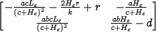
The stability of the system can be computed by evaluating eigenvalues of this matrix at different equilibrium points.
To explore how the parameters of the model affect the behavior of the
system, we choose to focus on two specific parameters of interest:
, the interaction coefficient between the populations and , a
parameter affecting the prey consumption rate.
Figure 4.17a is a numerically computed {\em
^{parametric stability diagram}} showing the regions in the chosen
parameter space for which the equilibrium point is stable (leaving the other
parameters at their nominal values).

|

|
|||
| (a) Stability diagram | (b) Bifurcation diagram | |||
|
Figure 4.17: Bifurcation analysis of
the predator-prey system. (a) Parametric stability diagram showing the
regions in parameter space for which the system is stable. (b)
Bifurcation diagram showing the location and stability
of the equilibrium point as a function of | ||||

We see from this figure that for certain combinations of
and we get a stable
equilibrium point, while at other values this equilibrium point is
unstable.
Figure 4.17b is a numerically computed
bifurcation diagram for the system. In this plot, we choose
one parameter to vary () and then plot the equilibrium value of
one of the states () on the vertical axis. The remaining
parameters are set to their nominal values. A solid line indicates
that the equilibrium point is stable; a dashed line indicates that the
equilibrium point is unstable. Note that the stability in the
bifurcation diagram matches that in the parametric stability diagram
for  (the nominal value) and varying from 1.35 to 4.
For the predator-prey system, when the equilibrium point is unstable,
the solution converges to a stable limit cycle. The amplitude of this
limit cycle is shown by the dashed-dotted line in
Figure 4.17b.
(the nominal value) and varying from 1.35 to 4.
For the predator-prey system, when the equilibrium point is unstable,
the solution converges to a stable limit cycle. The amplitude of this
limit cycle is shown by the dashed-dotted line in
Figure 4.17b.
MATLAB and Mathematica files:
- predprey_bif.mma - Mathematica file for doing symbolic calculations on the model
- predprey.mma - Mathematica file for doing symbolic calculations on the model
- Jac.m - Mathematica file computing the Jacobian of a vector field
- predprey_bif.m - MATLAB code to generate the bifurcation diagram
- predprey.dat - data file used for bifurcation diagram (generated by predprey.mma)
See the software page for more information on how to run these scripts.
State Feedback
Consider the problem of regulating the population of an ecosystem\index{ecosystems} by modulating the food supply. We use the predator--prey model introduced in Section Template:Sec:examples:predprey. The dynamics for the system are given by
We choose the following nominal parameters for the system, which correspond to the values used in previous simulations:
We take the parameter , corresponding to the growth rate for
hares, as the input to the system, which we might modulate by
controlling a food source for the hares. This is reflected in our
model by the term  in the first equation. We choose the
number of lynxes as the output of our system.
in the first equation. We choose the
number of lynxes as the output of our system.
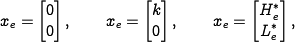
To control this system, we first linearize the system around the
equilibrium point of the system  , which can be determined
numerically to be
, which can be determined
numerically to be  . This yields a linear
dynamical system
. This yields a linear
dynamical system

where  ,
,  and
and  . It is easy to
check that the system is reachable around the equilibrium
. It is easy to
check that the system is reachable around the equilibrium  , and hence we can assign the eigenvalues of the system using
state feedback.
, and hence we can assign the eigenvalues of the system using
state feedback.
Determining the eigenvalues of the closed loop system requires
balancing the ability to modulate the input against the natural
dynamics of the system. This can be done by the process of trial and
error or by using some of the more systematic techniques discussed in
the remainder of the text. For now, we simply choose the desired
closed loop eigenvalues to be at  . We can then
solve for the feedback gains using the techniques described earlier,
which results in
. We can then
solve for the feedback gains using the techniques described earlier,
which results in
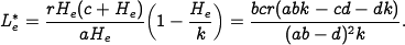
Finally, we solve for the reference gain  , using
equation~\eqref{eq:statefbk:kr} to obtain
, using
equation~\eqref{eq:statefbk:kr} to obtain  .
.
Putting these steps together, our control law becomes
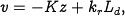
where  is the desired number of lynxes.
In order to implement the control law, we must rewrite it using the
original coordinates for the system, yielding
is the desired number of lynxes.
In order to implement the control law, we must rewrite it using the
original coordinates for the system, yielding
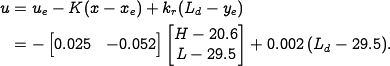
This rule tells us how much we should modulate as a function of
the current number of lynxes and hares in the ecosystem.
Figure 6.7a shows a simulation of the resulting
closed loop system using the parameters defined above and starting
with an
initial population of 15 hares and 20 lynxes.

|

|
|||
| (a) Initial condition response | (b) Phase portrait | |||
|
Figure 6.7: Simulation results for the controlled predator--prey system. The population of lynxes and hares as a function of time is shown in (a), and a phase portrait for the controlled system is shown in (b). Feedback is used to make the population stable at | ||||


Note that the system quickly stabilizes the population of lynxes at
the reference value ( ).
A phase portrait of the system is
given in Figure 6.7b, showing how other initial
conditions converge to the stabilized equilibrium population. Notice
that the dynamics are very different from the natural dynamics (shown
in Figure 3.20).
).
A phase portrait of the system is
given in Figure 6.7b, showing how other initial
conditions converge to the stabilized equilibrium population. Notice
that the dynamics are very different from the natural dynamics (shown
in Figure 3.20).
MATLAB files:
- predprey_control.m - MATLAB code to compute controllers via eigenvalue placement
- predprey.m - system definition (for use by ode45 and amphaseplot)
- predprey_rh.m - auxiliary files that define control law
See the software page for more information on how to run these scripts.