Robust Performance
| Prev: Frequency Domain Design | Chapter 12 - Robust Performance | Next: Bibliography |
This chapter focuses on the analysis of robustness of feedback systems. We consider the stability and performance of systems who process dynamics are uncertain and derive fundamental limits for robust stability and performance. We also discuss how to design controllers to achieve robust performance.
Textbook ContentsRobust Performance (pdf, 28Sep12)
|
Lecture Materials
Supplemental Information
|
Chapter Summary
This chapter focuses on the analysis of robustness of feedback systems:
Uncertainty can enter a model in many forms. Parametric uncertainty occurs when the values of the parameters in the model are not precisely known or may vary. Unmodeled dynamics are a more general class of uncertainty in which some portions of the systems behavior are not included in the model, either due to lack of knowledge or simplicity. Unmodeled dynamics can be taken into consideration by incorporating an uncertainty block with bounded input/output response. Common types of unmodeled dynamics include additive uncertainty, multiplicative uncertainty and feedback uncertainty.
The Vinnicombe metric (or
 -gap metric) provides a measure of the distance between two transfer functions. It is defined as
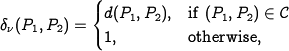
where
 is a distance measure between the two transfer function
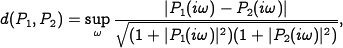
and
 is the set of all pairs
  such that the functions
  and
and  have the same number of zeros in the right half-plane.
Robust stability can be determined through the use of the Nyquist plot. The stability margin
 , defined as the shortest distance from -1 to the Nyquist curve, provides a measure of robustness. For an additive perturbation
  , the system is robustly stable if

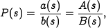
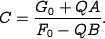
The Youla parameterization provides a description of all controllers that can stabilize a given process. For a stable system, stabilizing compensators are of the form

where
 is the process transfer function and
  is an arbitrary stable transfer function. For an unstable process, we write the process dynamics as
where
 and
and  are stable transfer functions. Stabilizing compensators have the form
where
 ,
,  and
and  are all stable transfer functions.
In addition to stability, uncertainty can also affect the performance of a system. For additive uncertainty, the load response satisfies

The response to load disturbances is thus insensitive to process variations for frequencies where the magnitude of the sensitivity function
 is small. Similarly, the response of the controller to noise in the presence of additive uncertainty satisfies
indicating that the controller is insensitive to noise when the complementary sensitivity is small. Control design in the presence of uncertainty can be done by using the Gang of Four to ensure that the appropriate sensitivity functions are all well behaved.
State space design, using eigenvalue (or pole) placement, can also be analyzed using sensitivity functions. State space design is complicated in the presence of right half plane poles and zeros, which limit the achievable performance. Design rules for robust pole placement include:
- Slow stable process zeros should be matched by slow closed loop poles
- Fast stable process poles should be matched by fast closed loop poles
- Slow unstable process zeros and fast unstable process poles impose performance limitations
Design methods for robust stability performance include quantitative feedback theory (QFT), linear quadratic control (LQG) and and
 control. Strong robustness results are available for control. Letting
  represent the input/output response between a set of generalized disturbances
  and the generalized error
  , it can be shown that
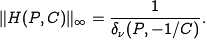
The Vinnecombe metric can thus be considered as a generalized stability margin (comparable to
) and it follows that if we find a controller  with
with 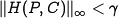 , then this controller will stabilize any process
  such that
 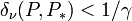 .
.
This condition can be derived using the small gain theorem and allows us to reason about uncertainty without exact knowledge of the process perturbations.
Frequently Asked Questions
Errata
|
MATLAB codeThe following MATLAB scripts are available for producing figures that appear in this chapter.
See the software page for more information on how to run these scripts. |