Dynamic Behavior
| Prev: Examples | Chapter 4 - Dynamic Behavior | Next: Linear Systems |
In this chapter we give a broad discussion of the behavior of dynamical systems, focused on systems modeled by nonlinear differential equations. This allows us to discuss equilibrium points, stability, limit cycles and other key concepts of dynamical systems. We also introduce some methods for analyzing global behavior of solutions.
Textbook ContentsDynamic Behavior (pdf, 28Sep12)
|
Lecture MaterialsSupplemental Information
|
Chapter Summary
This chapter introduces the basic concepts and tools of dynamical systems.
-
We say that
 is a solution of a differential equation on the time interval
  to
to  with initial value
  if it satisfies

 . For most differential equations we will encounter, there is a unique solution for a given initial condition. Numerical tools such as MATLAB and Mathematica can be used to obtain numerical solutions for given the function
  .
. An equilibrium point for a dynamical system represents a point
 such that if
  then
then  for all
  . Equilibrium points represent stationary conditions for the dynamics of a system. A limit cycle for a dynamical system is a solution which is periodic with some period
  , so that
  for all .
An equilibrium point is (locally) stable if initial conditions that start near an equilibrium point stay near that equilibrium point. A equilibrium point is (locally) asymptotically stable if it is stable and, in addition, the state of the system converges to the equilibrium point as time increases. An equilibrium point is unstable if it is not stable. Similar definitions can be used to define the stability of a limit cycle.
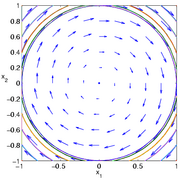
Phase portraits provide a convenient way to understand the behavior of 2-dimensional dynamical systems. A phase portrait is a graphical representation of the dynamics obtained by plotting the state
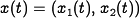 in the plane. This portrait is often augmented by plotting an arrow in the plane corresponding to , which shows the rate of change of the state. The following diagrams illustrate the basic features of a dynamical systems:
An asymptotically stable equilibrium point at  .
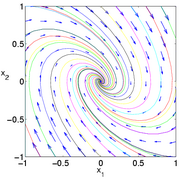
.A limit cycle of radius one, with an unstable equilibrium point at  .
.A stable equlibirum point at (nearby initial conditions stay nearby).A linear system

is asymptotically stable if and only if all eigenvalues of
 all have strictly negative real part and is unstable if any eigenvalue of has strictly positive real part. A nonlinear system can be approximated by a linear system around an equilibrium point by using the relationship
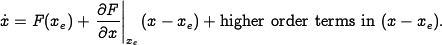
Since
 , we can approximate the system by choosing a new
state variable
, we can approximate the system by choosing a new
state variable  and writing the dynamics as
  . The stability of the nonlinear system can be determined in a local neighborhood of the equilibrium point through its linearization.
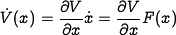
A Lyapunov function is an energy-like function
 that can be used to reason about the stability of an equilibrium point. We define the derivative of
  along the trajectory of the system as
Assuming
 and
and  , the following conditions hold:
Condition on Condition on 
Stability 
 for all
  stable

 asymptotically stable
Stability of limit cycles can also be studied using Lyapunov functions.
The Krasovskii-LaSalle Principle allows one to reason about asymptotic stability even if the time derivative of
is only negative semi-definite ( rather than
  ). Let be a positive definite function,
  for all
  and , such that
on the compact set
and , such that
on the compact set  .
.
Then as
 , the trajectory of the system will converge to the largest invariant set inside
 .
.In particular, if
 contains no invariant sets other than
  , then 0 is asymptotically stable.
The global behavior of a nonlinear system refers to dynamics of the system far away from equilibrium points. The region of attraction of an asymptotically stable equilirium point refers to the set of all initial conditions that converge to that equilibrium point. An equilibrium point is said to be globally asymptotically stable if all initial conditions converge to that equilibrium point. Global stability can be checked by finding a Lyapunov function that is globally positive definition with time derivative globally negative definite.


