Transfer Functions

Chapter 8 - Transfer Functions

This chapter introduces the concept of the transfer function, which is a compact description of the input-output relation for a linear system. Combining transfer functions with block diagrams gives a powerful method of dealing with complex systems. The relationship between transfer functions and other system descriptions of dynamics is also discussed.

Textbook Contents

Transfer Functions (pdf, 28Sep12)

1. Frequency Domain Analysis
2. Derivation of the Transfer Function
3. Block Diagrams and Transfer Functions
4. The Bode Plot
5. Transfer Functions from Experiments
6. Laplace Transforms
7. Further Reading
8. Exercises

Lecture Materials

Supplemental Information

Chapter Summary

This chapter introduces the concept of a transfer functon for a linear input/output system.

The frequency response of a linear system

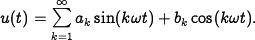
is the response of the system to a sinusoidal input at a given frequency. Due to linearity, the response of a system to a more complicated input can be constructed by decomposing the input into the sum of sines and cosines

(The frequency response is described in Chapter 5 - Linear Systems).
More, generally an exponential signal is given by

where $\text{[math]}$ gives the decay rate of the signal and $\text{[math]}$ is the oscillation frequency of the signal. The response to an exponential signal is given by
The transfer function for a linear system is given by

The transfer function represents the steady state response of the system to an exponential input. The transfer function is independent of the choice of coordinates for the state space.
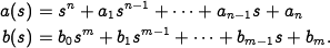
The transfer function for a linear differential equation of the form

is given by

where
The zero frequency gain of a system is given by the magnitude of the transfer function at $\text{[math]}$ . It represents the ratio of the steady state value of the output with respect to a step input. For a transfer function of the form 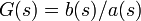$\text{[math]}$ , the roots of the polynomial $\text{[math]}$ are called the poles of the system and the roots of the polynomial $\text{[math]}$ are called the zeros of the system. A pole $\text{[math]}$ is also called a mode of the system. The poles correspond to the eigenvalues of the dynamics matrix $\text{[math]}$ and determine the stability of the system. The zeros of a transfer function correspond to exponential signals whose transmission is blocked by the system.
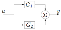
Block diagrams that consist of transfer functions can be manipulated using block diagram algebra. The following table gives the transfer functions for some common interconnections of linear systems

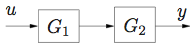
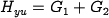
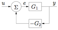
Series: Parallel: Feedback: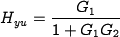
A Bode plot is a plot of the magnitude and phase of the frequency response:

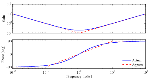
The top plot is the gain curve; the frequency and magnitude are both plotted using a logarithmic scale. The bottom plot is the phase curve and uses a log-linear scale. The dashed lines show straight line approximations of the gain curve and the corresponding phase curve.
The transfer function for a system can be determined from experiments by measuring the frequency response and fitting a transfer function to the data. Formally, the transfer function corresponds to the ratio of the Laplace transforms of the output to the input.