Frequency Domain Design

Chapter 11 - Frequency Domain Design

In this chapter we continue to explore the use of frequency domain techniques for design of feedback systems. We begin with a more thorough description of the performance specifications for controls systems, and then introduce the concept of "loop shaping" as a mechanism for designing controllers in the frequency domain. We also introduce some fundamental limitations to performance for systems with right half plane poles and zeros.

Textbook Contents

Frequency Domain Design (pdf, 28Sep12)

1. A Basic Feedback Loop
2. Performance Specifications
3. Feedback Design via Loop Shaping
4. Fundamental Limitations
5. Design Example
6. Further Reading
7. Exercises

Lecture Materials

Lectures: Loop Shaping, Limits of Performance
Additional Exercises

Supplemental Information

Chapter Summary

This chapter describes the use of the loop shaping to design a control law to achieve a desired level of performance:

Control design in the frequency domain consists of designing a feedback controller $\text{[math]}$ and a feedforward controller $\text{[math]}$ as illustrated in the basic feedback diagram below:

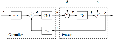
The external signals are the reference signal $\text{[math]}$ , the load disturbance $\text{[math]}$ and the measurement noise $\text{[math]}$ . The process output is $\text{[math]}$ , and the control signal is $\text{[math]}$ . This control structure is also known as a two degree of freedom controller.
The primary transfer functions that define the input/output characteristics of the system are called the Gang of Six:

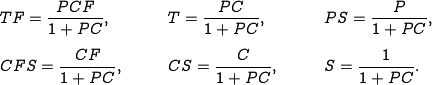
The transfer functions in the first column give the response of the process output and control signal to the reference signal. The second column gives the response of the control variable to the load disturbance and the noise, and the final column gives the response of the process output to those two inputs. When $\text{[math]}$ , the system is said to have pure error feedback and the relevant input/output transfer functions are given by the Gang of Four, given by the transfer functions in the right two columns.
Feedforward compensation is used to provided improved response to reference signals and measured disturbances (2 DOF system). The figure below illustrates one possible structure for designing a feedforward compensator:

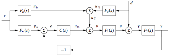
Three feedforward elements are present: $\text{[math]}$ sets the desired output value, $\text{[math]}$ generates the feedforward command $\text{[math]}$ and $\text{[math]}$ attempts to cancel disturbances. The transfer function from reference input to process output is given by

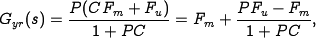
The first term represents the desired transfer function and the second term should be made small. Perfect feedforward compensation is obtained by choosing $\text{[math]}$ .
The performance of a system can be given in terms of the characteristics of the frequency response between an input and output. A resonant peak is a maximum of the gain, and the peak frequency is the corresponding frequency. The gain crossover frequency is the frequency where the open loop gain is equal one. The bandwidth is defined as the frequency range where the closed loop gain is of the low-frequency gain (low-pass), mid-frequency gain (band-pass) or high-frequency gain (high-pass).
The sensitivity function 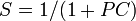$\text{[math]}$ describes how disturbances are attenuated by closing the feedback loop. Disturbances with frequencies such that $\text{[math]}$ are attenuated, but disturbances with frequencies such that $\text{[math]}$ are amplified by feedback. The maximum sensitivity $\text{[math]}$ , which occurs at the frequency $\text{[math]}$ , is a measure of the largest amplification of the disturbances. The complementary sensitivity function 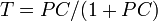$\text{[math]}$ describes how well the controller tracks a references signal. The maximum complementary sensitivity, $\text{[math]}$ , which occurs at the frequency $\text{[math]}$ , is the peak value of the magnitude of the complementary sensitivity function. It provides the maximum amplification from the reference signal to the output signal.
There are approximate relations between specifications in the time and frequency domains. In the frequency domain the response time can be characterized by the closed loop bandwidth $\text{[math]}$ , the gain crossover frequency $\text{[math]}$ and the sensitivity frequency $\text{[math]}$ . The product of bandwidth and rise time is approximately constant, , so decreasing the rise time corresponds to increasing the closed loop bandwidth. The overshoot of the step response $\text{[math]}$ is related to the resonant peak $\text{[math]}$ of the frequency response in the sense that a larger peak normally implies a larger overshoot.
Using frequency domain specifications, controllers can often be designed by shaping the loop transfer function, $\text{[math]}$ . The gain curve and sensitivity functions for a typical loop transfer function are shown below:

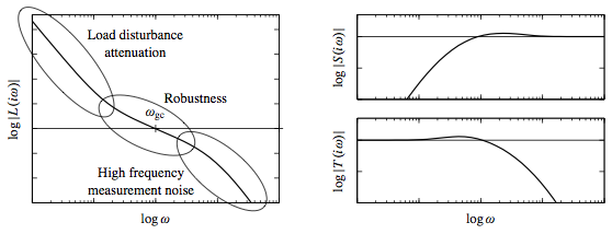
The plot on the left shows the gain curve and the plots on the right show the sensitivity function and complementary sensitivity function. The gain crossover frequency $\text{[math]}$ and the slope $\text{[math]}$ of the gain curve at crossover are important parameters that determine the robustness of closed loop systems. At low frequency, a large magnitude for $\text{[math]}$ provides good load disturbance rejection and reference tracking, while at high frequency a small loop gain is used to avoid amplifying measurement noise.
A common control element to shape the loop transfer function is to use a pole/zero pair:

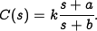
The compensator is called a lead compensator if $\text{[math]}$ the controller provides phase lead between frequencies $\text{[math]}$ and $\text{[math]}$ . The compensator is called a lag compensator if $\text{[math]}$ and this form is often used to provide low frequency gain. Lead and lag compensation are closely related to PD and PI controllers.
Feedback control systems have a number of fundamental limits, usually exacerbated by the presence of right half plane poles and zeros. For systems with right half plane poles or zeros, we can decompose the process dynamics into a minimum phase transfer function (no right half plane poles or zeros) and an all pass transfer function (gain = 1):

The gain crossover inequality

provides a relationship between the phase margin , the slope of the gain curve $\text{[math]}$ . For processes with near pole/zero cancellations in the right half plane, the gain crossover inequality limits the maximum amount of achievable phase margin.
Another fundamental limit is given by Bode's integral formula, which states that for systems with a loop transfer function that goes to zero faster than $\text{[math]}$ as , the sensitivity function must satisfy

where $\text{[math]}$ are the poles in the right half-plane. This conservation law shows that to get lower sensitivity in one frequency range, we must get higher sensitivity in some other region. An analogous formula exists for the complementary sensitivity function in the presence of right half plane zeros.