FAQ: What does the Nyquist plot look like for a system with poles at the origin?

Section 9.2 and Example 9.2 in the main text describe how to sketch the Nyquist plot for a system with a pole at the origin. In general, when there are poles at the origin (or any other point along the imaginary axis), a small semi-circle is drawn to the right of the pole, creating a large circle in the Nyquist plot, as shown below:

	Figure 9.3a: Nyquist D contour		Figure 9.5b: Nyquist plot

The dash-dotted portion of the Nyquist plot on the right corresponds to the small semicircle of radius at the origin.

Figuring out which way the Nyquist plot closes for a single pole at the origin

For a single pole at the origin, the Nyquist curve will approach infinity as approaches zero from both the positive and negative direction. The Nyquist curve can then be "closed" by tracing around a small semicircle to the left of the pole (as shown in Figure 9.3a). The small semicircle will attach the two ends of the Nyquist curve at infinity by creating a large semicircle joining the two ends of the Nyquist curve. The stability of the system will often depend on whether this large semi-circle is on the right or the left of the complex plane.

A simple way to determine on which side the Nyquist plot is closed is to evaluate the transfer function at , where is a small, positive, real number. The transfer function will be real-valued if is real and if then the Nyquist plot closes on the right, otherwise on the left. This trick only works for poles at the origin and only works if there is a single pole at the origin.

Multiple poles at the origin

When there are multiple poles at the origin, the magnitude of the Nyquist curve still goes to infinity near zero frequency, but one has to be more careful in determining how to close the curve. The proper way to do this is to explicitly evaluate the Nyquist curve along a semi-circle of radius . If we let represent the portion of the Nyquist contour near the origin and represent the corresponding portion of the Nyquist plot, then we have:

If is chosen sufficiently small, then the only -dependent contribution to the Nyquist curve will be due to the poles at the origin. In this case, we can writ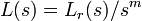e where is the portion of the loop transfer function that has no poles at the origin and is the number of open loop poles at the origin. It follows that

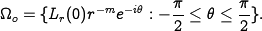
The contour consists of semicircles and hence we get one complete encirclement for every two poles at the origin. The direction of the encirclement is in the clockwise direction (since is a counterclockwise oriented segment, as shown in Figure 9.3a).

Note that if you have an odd number of poles, the two "ends" of the Nyquist curve (for positive and negative values on the axis) will be 180 degrees apart. If you have an even number of poles, the two "ends" of the Nyquist curve will both be real and you "connect" the ends by going around in one or more complete circles. To see these effects, try drawing Nyquist curves for the following transfer functions: