 |
Lecture 3.1: Stability and
Performance
14 October 2002
|
 |
 This
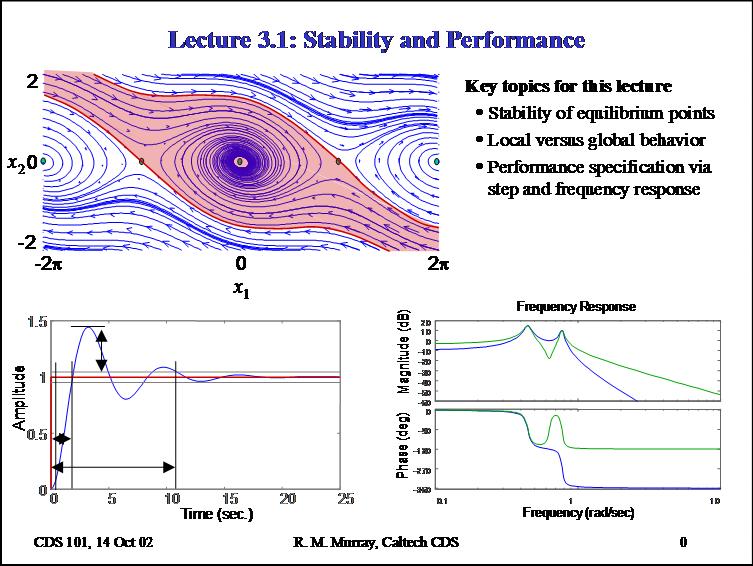
lecture provides and introduction to stability and performance of (nonlinear)
control systems. A formal definition of stable systems is given and phase portraits
are introduced to help visualize the concepts. Local and global behavior of
nonlinear systems is discussed, using a damped pendulum and the preditor-prey
problem as examples. Performance of control systems is presented for both transient
(step respones) and steady state (frequency domain) specifications.
This
lecture provides and introduction to stability and performance of (nonlinear)
control systems. A formal definition of stable systems is given and phase portraits
are introduced to help visualize the concepts. Local and global behavior of
nonlinear systems is discussed, using a damped pendulum and the preditor-prey
problem as examples. Performance of control systems is presented for both transient
(step respones) and steady state (frequency domain) specifications.
Mud card responses [advanced
search]:
#!/usr/bin/perl
# -*- perl -*-
#
# htdbsearch.cgi - search for matching files in a database directory
# RMM, 16 Mar 97
#
# This CGI script searches the description files in a directory for a
# against a set of criteria
#
# This script should be called as
#
# http://machine/path/htdblist.cgi?
# or
# http://machine/path/htdblist.cgi?db=&args
#
# where is the name of the configuration file that defines
# all of the information needed to generate the listing. The optional
# arguments are:
#
# _count=NN only list the first NN entries
# _tight=1 use tight listing
# _ssi=1 don't print header, trailer info (for includs)
#
# Include the necessary libraries
require "cgi-lib.pl";
require "htdblib.pl";
# Parse script arguments
if (&htdbinit) {
# If the form contains some values, use them to search, and return
# the results.
if ($in{'_dbconfig'}) {
# Generate the context header for the browser
print &PrintHeader;
# Print out the introductory information for search
if (defined &SearchHeader) {&{$SearchHeader}($DBName);}
# Summarize the search that was performed
$rsltheader =
defined &ResultHeader ? \&ResultHeader : htdb::ResultHeader;
&{$rsltheader}(%in) if (!$in{_ssi});
# Go through and look for matching files
if (not &PrintMatches) { &PrintNoMatches if (!in{ssi}); }
# Generate the trailer
if (defined &dbtrailer) {$dbtrailer = \&DBTrailer};
if (not $dbtrailer) {$dbtrailer = \&htdb::DBTrailer;}
&{$dbtrailer}($DBName) if (!in{ssi});
} else {
# Check to see if there is a user function for printing the search form
if (defined &SearchForm) {$searchform = \&SearchForm};
if (not $searchform) {$searchform = \&htdb::SearchForm;}
# Print out the introductory information for search
if (defined &SearchHeader) {&{$SearchHeader}($DBName);}
# Print the search form
&{$searchform}(%in);
}
}
#
# Subroutine for printing the matches that occured
#
sub PrintMatches {
my ($num_found);
# Go to the database directory and read the contents
chdir $DBPath || die "Can't cd to $DBPath";
opendir(DIR, '.') || die "Can't open $DBPath";
@filenames = readdir(DIR);
closedir(DIR);
# Check to see if there is a user function for checking matches
if (defined &CheckEntry) {$checkentry = \&CheckEntry};
if (not $checkentry) {$checkentry = \&htdb::CheckEntry;}
# Check to see if there is a user function for parsing filenames
if (defined &ParseFname) {$parsefname = \&ParseFname};
if (not $parsefname) {$parsefname = \&htdb::ParseFname;}
# Check to see if there is a user function for printing the entry
if (defined &PrintEntry) {$printentry = \&PrintEntry};
if (not $printentry) {$printentry = \&htdb::PrintEntry;}
# Check to see if there is a user function for printing the entry
if (defined &TightEntry) {$tightentry = \&TightEntry};
if (not $tightentry) {$tightentry = \&htdb::TightEntry;}
# Open the list environment used for the results
# Print the command to generate a list of elements
print ($in{_tight} ? "\n" : "\n");
# Loop through the filenames in order.
$getfnames = defined &GetFnames ? \&GetFnames : htdb::GetFnames;
@filenames = &{$getfnames}($DBPath);
for (@filenames) {
# Parse the filname and extract the ID and tag information
($id, $tag) = &{$parsefname}($filename = $_);
next if not $id;
# Open the file and extract the contents
$contents = &htdb::readfile($filename);
next if not $contents;
# Now see if this entry matches the criteria for a match
next if not &{$checkentry}($contents, %in);
# Print out the information associated with this entry
$count += &{($in{_tight} ? $tightentry : $printentry)}
($filename, $contents, $id, $tag, $DBURL."/".$filename);
$num_found++;
# See if we are counting and stop if needed
last if ($in{_count} && $count > $in{_count});
}
# Close the list environment used for the results
print ($in{_tight} ? "
\n" : "\n");
return $num_found;
}
#
# Subroutine for alerting the user that no matches occured
#
sub PrintNoMatches {
print "No matches found
\n";
print "Sorry, no entries match your request. ";
print "Please choose some different parameters and try again.\n";
print $footer;
}
Handouts from lecture
The following materials were handed out in lecture. These have been updated to
include any corrections.
Required reading
Supplemental reading
This homework set covers stability and performance through a series of application
examples. The first problem provides a set of three real-world models in which
the student must identify the equilibrium points and determine stability of
the equilibrium points (through simulation). The second problem explores performance
specification in the conext of the cruise control example, including step response
and frequency response.
Modifications to the homework (link above is always the latest version):
- 19 Oct 02: minor changes to fix typos and clarify some statements
- Step response in 2(a) should be from 55 to 65 mph
- Frequency in 2(b) should be 1 Hz (about 6 rad/sec)
- Problem 3(a) had some information which was not correct. It has been
modified and the initial condition has been changed from y(0) = -1 to
y(0) = 1.
- 16 Oct 02: handed out remaining problems (CDS 110)
- 14 Oct 02: handed out first two problems
Frequently asked questions on homework and TA hints:
#!/usr/bin/perl
# -*- perl -*-
#
# htdbsearch.cgi - search for matching files in a database directory
# RMM, 16 Mar 97
#
# This CGI script searches the description files in a directory for a
# against a set of criteria
#
# This script should be called as
#
# http://machine/path/htdblist.cgi?
# or
# http://machine/path/htdblist.cgi?db=&args
#
# where is the name of the configuration file that defines
# all of the information needed to generate the listing. The optional
# arguments are:
#
# _count=NN only list the first NN entries
# _tight=1 use tight listing
# _ssi=1 don't print header, trailer info (for includs)
#
# Include the necessary libraries
require "cgi-lib.pl";
require "htdblib.pl";
# Parse script arguments
if (&htdbinit) {
# If the form contains some values, use them to search, and return
# the results.
if ($in{'_dbconfig'}) {
# Generate the context header for the browser
print &PrintHeader;
# Print out the introductory information for search
if (defined &SearchHeader) {&{$SearchHeader}($DBName);}
# Summarize the search that was performed
$rsltheader =
defined &ResultHeader ? \&ResultHeader : htdb::ResultHeader;
&{$rsltheader}(%in) if (!$in{_ssi});
# Go through and look for matching files
if (not &PrintMatches) { &PrintNoMatches if (!in{ssi}); }
# Generate the trailer
if (defined &dbtrailer) {$dbtrailer = \&DBTrailer};
if (not $dbtrailer) {$dbtrailer = \&htdb::DBTrailer;}
&{$dbtrailer}($DBName) if (!in{ssi});
} else {
# Check to see if there is a user function for printing the search form
if (defined &SearchForm) {$searchform = \&SearchForm};
if (not $searchform) {$searchform = \&htdb::SearchForm;}
# Print out the introductory information for search
if (defined &SearchHeader) {&{$SearchHeader}($DBName);}
# Print the search form
&{$searchform}(%in);
}
}
#
# Subroutine for printing the matches that occured
#
sub PrintMatches {
my ($num_found);
# Go to the database directory and read the contents
chdir $DBPath || die "Can't cd to $DBPath";
opendir(DIR, '.') || die "Can't open $DBPath";
@filenames = readdir(DIR);
closedir(DIR);
# Check to see if there is a user function for checking matches
if (defined &CheckEntry) {$checkentry = \&CheckEntry};
if (not $checkentry) {$checkentry = \&htdb::CheckEntry;}
# Check to see if there is a user function for parsing filenames
if (defined &ParseFname) {$parsefname = \&ParseFname};
if (not $parsefname) {$parsefname = \&htdb::ParseFname;}
# Check to see if there is a user function for printing the entry
if (defined &PrintEntry) {$printentry = \&PrintEntry};
if (not $printentry) {$printentry = \&htdb::PrintEntry;}
# Check to see if there is a user function for printing the entry
if (defined &TightEntry) {$tightentry = \&TightEntry};
if (not $tightentry) {$tightentry = \&htdb::TightEntry;}
# Open the list environment used for the results
# Print the command to generate a list of elements
print ($in{_tight} ? "\n" : "\n");
# Loop through the filenames in order.
$getfnames = defined &GetFnames ? \&GetFnames : htdb::GetFnames;
@filenames = &{$getfnames}($DBPath);
for (@filenames) {
# Parse the filname and extract the ID and tag information
($id, $tag) = &{$parsefname}($filename = $_);
next if not $id;
# Open the file and extract the contents
$contents = &htdb::readfile($filename);
next if not $contents;
# Now see if this entry matches the criteria for a match
next if not &{$checkentry}($contents, %in);
# Print out the information associated with this entry
$count += &{($in{_tight} ? $tightentry : $printentry)}
($filename, $contents, $id, $tag, $DBURL."/".$filename);
$num_found++;
# See if we are counting and stop if needed
last if ($in{_count} && $count > $in{_count});
}
# Close the list environment used for the results
print ($in{_tight} ? "
\n" : "\n");
return $num_found;
}
#
# Subroutine for alerting the user that no matches occured
#
sub PrintNoMatches {
print "No matches found
\n";
print "Sorry, no entries match your request. ";
print "Please choose some different parameters and try again.\n";
print $footer;
}