Vectored thrust aircraft

This page documents the (planar) vertical takeoff and landing (PVTOL) aircraft model that is used as a running example throughout the text. A detailed description of the dynamics of this system is presented in Chapter 2 - System Modeling, with control analysis and design performed in Chapter 6 - State Feedback and Chapter 11 - Frequency Domain Design. This page brings together this material into a single place, to illustrate the application of analysis and design tools for this system. Links to MATLAB scripts are included that generate the analysis and figures described here.

System Description

Consider the motion of vectored thrust aircraft, such as the Harrier "jump jet" shown below (left). The Harrier AV-8B military aircraft redirects its engine thrust downward so that it can "hover" above the ground. Some air from the engine is diverted to the wing tips to be used for maneuvering.

A simplified model of the Harrier is shown above (right), where we focus on the motion of the vehicle in a vertical plane through the wings of the aircraft. We resolve the forces generated by the main downward thruster and the maneuvering thrusters as a pair of forces and acting at a distance below the aircraft (determined by the geometry of the thrusters).

Let denote the position and orientation of the center of mass of the aircraft. Let be the mass of the vehicle, the moment of inertia, the gravitational constant and the damping coefficient. Then the equations of motion for the vehicle are given by

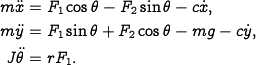
It is convenient to redefine the inputs so that the origin is an equilibrium point of the system with zero input. Letting and , the equations become

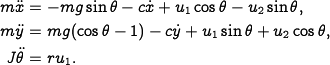
These equations describe the motion of the vehicle as a set of three coupled second-order differential equations.

LQR state feedback controller

This section demonstrates the design of an LQR state feedback controller for the vectored thrust aircraft example. This example is pulled from Chapter 6 - State Feedback.

• pvtol_lqr.m - MATLAB code used to produce figures in this example
• pvtol_params.m - parameter definitions

See the software page for more information on how to run these scripts.

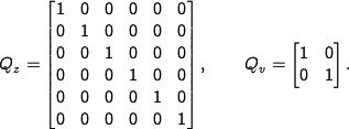
The dynamics of the system can be written in state space form as

Parameter Value Comment 4 kg system mass 0.0475 kg m^2 system inertia 0.25 m thrust offset 9.8 m/s gravitational constant 0.05 N s/m rotational damping

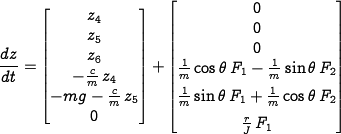
The system parameters are shown at the right and correspond to a scaled model of the system. The equilibrium point for the system is given by , and 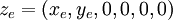. To derive the linearized model near an equilibrium point, we compute the linearization at

Letting and , the linearized system is given by

It can be verified that the system is reachable.

To compute a linear quadratic regulator for the system, we write the cost function as

where and represent the local coordinates around the desired equilibrium point . We begin with diagonal matrices for the state and input costs:

This gives a control law of the form , which can then be used to derive the control law in terms of the original variables:

The equilibrium points have 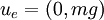and . The response of the closed loop system to a step change in the desired position is shown below.

Step response in and		Effect of control weight

The plot on the left shows the and positions of the aircraft when it is commanded to move 1 m in each direction. The response can be tuned by adjusting the weights in the LQR cost. The plot on the right shows the motion for control weights , , . A higher weight of the input term in the cost function causes a more sluggish response.

Lateral control using inner/outer loop design

To control the lateral dynamics of the vectored thrust aircraft, we make use of a "inner/outer" loop design methodology. This example is drawn from Chapter 11 - Frequency Domain Design.

• pvtol_nested.m - MATLAB code used to produce figures in this example
• pvtol_params.m - parameter definitions

We begin by representing the dynamics using the block diagram

where

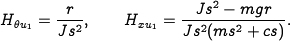
The controller is constructed by splitting the process dynamics and controller into two components: an inner loop consisting of the roll dynamics and control and an outer loop consisting of the lateral position dynamics and controller .

The closed inner loop dynamics control the roll angle of the aircraft using the vectored thrust while the outer loop controller commands the roll angle to regulate the lateral position. As a performance specification for the entire system, we would like to have zero steady-state error in the lateral position, a bandwidth of approximately 1 rad/s and a phase margin of 45°.

Inner loop design

For the inner loop, we choose our design specification to provide the outer loop with accurate and fast control of the roll. The inner loop dynamics are given by

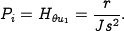
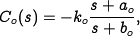
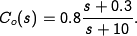
We choose the desired bandwidth to be 10 rad/s (10 times that of the outer loop) and the low-frequency error to be no more than 5%. To achieve our performance specification, we would like to have a gain of at least 10 at a frequency of 10 rad/s, requiring the gain crossover frequency to be at a higher frequency. We see from the loop shape below (left) that in order to achieve the desired performance we cannot simply increase the gain since this would give a very low phase margin. Instead, we must increase the phase at the desired crossover frequency.

Open loop roll dynamics	Loop transfer function with lead compensator	Closed loop roll dynamics

To accomplish this, we use a lead compensator with and :

We then set the gain of the system to provide a large loop gain up to the desired bandwidth, as shown above (center). We see that this system has a gain of greater than 10 at all frequencies up to 10 rad/s and that it has more than 60° of phase margin.

The resulting closed loop dynamics for the system satisfy

A plot of the magnitude of this transfer function is shown above (right), and we see that is a good approximation up to 10 rad/s.

Outer loop design

To design the outer loop controller, we assume the inner loop roll control is perfect, so that we can take as the input to our lateral dynamics. The outer loop dynamics can be written as

where we replace with to reflect our approximation that the inner loop will eventually track our commanded input. Of course, this approximation may not be valid, and so we must verify this when we complete our design.

Our control goal is now to design a controller that gives zero steady-state error in and has a bandwidth of 1 rad/s. The outer loop process dynamics are given by a second-order integrator, and we can again use a simple lead compensator to satisfy the specifications. We also choose the design such that the loop transfer function for the outer loop has for rad/s, so that the dynamics can be neglected. We choose the controller to be of the form

with the negative sign to cancel the negative sign in the process dynamics. To find the location of the poles, we note that the phase lead flattens out at approximately . We desire phase lead at crossover, and we desire the crossover at rad/s, so this gives . To ensure that we have adequate phase lead, we must choose such that , which implies that should be between 0.1 and 1. We choose . Finally, we need to set the gain of the system such that at crossover the loop gain has magnitude 1. A simple calculation shows that satisfies this objective. Thus, the final outer loop controller becomes

Complete system analysis

Finally, we can combine the inner and outer loop controllers and verify that the system has the desired closed loop performance. The Bode and Nyquist plots with inner and outer loop controllers are shown below Figure~\ref{fig:pvtol:nested-plots}, and we see that the specifications are satisfied.

Bode plot for combined controller	Nyquist plot for combined controller	Zoomed in Nyquist plot

The system has a phase margin of 68° a gain margin of 6.2.

To better understand the properties of the closed loop system, we can generate the Gang of Four:

We see that the transfer functions between all inputs and outputs are reasonable. The sensitivity to load disturbances is large at low frequency because the controller does not have integral action.

The approach of splitting the dynamics into an inner and an outer loop is common in many control applications and can lead to simpler designs for complex systems. Indeed, for the aircraft dynamics studied in this example, it is very challenging to directly design a controller from the lateral position to the input . The use of the additional measurement of greatly simplifies the design because it can be broken up into simpler pieces.