Queuing systems
A common process in computing systems (and web servers) is managing a queue of requests. Typical queues can either by first-in, first-out (FIFO) or last-in, first-out (LIFO). The most common for web servers is the FIFO queue.
Modeling

A schematic diagram of a simple queue is shown to the right. Messages arrive at rate  and are stored in a queue. Messages are processed and removed from the queue at rate
  . The average size of the queue is given by
  . There can be large variations in arrival rates and service rates, and the queue length builds
up when the arrival rate is larger than the service rate. When the queue becomes too large, service is denied using an admission control
policy.
. There can be large variations in arrival rates and service rates, and the queue length builds
up when the arrival rate is larger than the service rate. When the queue becomes too large, service is denied using an admission control
policy.
The system can be modeled in many different ways. One way is to model each incoming request, which leads to an event-based model where the state is an integer that represents the queue length. The queue changes when a request arrives or a request is serviced. A discrete-time model that captures these dynamics is given by the difference equation

where  and
and  are random variables
representing incoming and outgoing requests on the queue. These
variables take the values 0 or 1 with some probability at each time
instant. In many cases it is possible
to determine statistics
of quantities like queue length and service time, but the computations can be
quite complicated.
To capture the statistics of the arrival and servicing of messages,
we model each of these as a {\em Poisson process} in which the
number of events occurring in a fixed time has a given rate, with
the specific timing of events independent of the time since the last
event. (The details of random processes are beyond the scope of this
text, but can be found in standard texts such as [Pit99].)
are random variables
representing incoming and outgoing requests on the queue. These
variables take the values 0 or 1 with some probability at each time
instant. In many cases it is possible
to determine statistics
of quantities like queue length and service time, but the computations can be
quite complicated.
To capture the statistics of the arrival and servicing of messages,
we model each of these as a {\em Poisson process} in which the
number of events occurring in a fixed time has a given rate, with
the specific timing of events independent of the time since the last
event. (The details of random processes are beyond the scope of this
text, but can be found in standard texts such as [Pit99].)
A significant simplification can be obtained by using a flow
model. Instead of keeping track of
each request we instead
view service and requests as flows, similar to what is done when
replacing molecules by a continuum when analyzing fluids. Assuming that
the average queue length  is a continuous variable and that
arrivals and
services are
flows with rates and , the
system can be modeled by the first-order differential equation
is a continuous variable and that
arrivals and
services are
flows with rates and , the
system can be modeled by the first-order differential equation
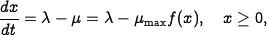
where  is the maximum service rate and
  is a number
between 0 and 1 that describes the effective service rate as a
function of the queue length.
is a number
between 0 and 1 that describes the effective service rate as a
function of the queue length.
It is natural to assume that the effective service rate depends on the
queue length because larger queues require more
resources. In steady
state we have 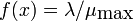 , and we assume that the queue
length goes to zero when
, and we assume that the queue
length goes to zero when  goes to zero and that it
goes to infinity when goes to 1. This implies that
goes to zero and that it
goes to infinity when goes to 1. This implies that
 and that
  . In addition, if we assume that the
effective service rate deteriorates monotonically with queue length,
then the function is monotone and concave. A simple function
that satisfies the basic requirements is
. In addition, if we assume that the
effective service rate deteriorates monotonically with queue length,
then the function is monotone and concave. A simple function
that satisfies the basic requirements is 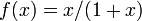 , which gives
the model (FAQ)
, which gives
the model (FAQ)
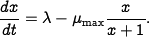
This model was proposed by Agnew~\cite{Agnew76}. It can be shown that if arrival and service processes are Poisson processes, the average queue length is given by equation~\eqref{eq:webserv:webseverdynamics} and that equation~\eqref{eq:webserv:webseverdynamics} is a good approximation even for short queue lengths; see Tipper~\cite{Tip+Sun90}.
To explore the properties of the model we will first investigate the
equilibrium value of the queue length when the arrival rate is
constant. Setting the derivative  to zero
in the dynamics and solving for , we
find that the queue length approaches the steady-state value
to zero
in the dynamics and solving for , we
find that the queue length approaches the steady-state value
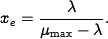

The figure to the right shows the steady-state queue
length as a function of , the effective service
rate excess.
Notice that the queue length increases rapidly as
approaches . To have a queue length less than 20
requires  . The average time to service a
request is
. The average time to service a
request is  , and it increases dramatically as
approaches .
, and it increases dramatically as
approaches .

The next figure illustrates the behavior of the server
in a typical overload situation.
The solid line shows a realization of an event-based
simulation, and the dashed line shows the behavior of the flow
model.
The maximum service rate is
 , and the arrival rate starts at
  . The
arrival rate is increased to
. The
arrival rate is increased to  at time 20, and it returns to
at time 25. The figure shows that the queue builds up
quickly and clears very slowly. Since the response time is
proportional to queue length, it means that the quality of service is
poor for a long period after an overload. This behavior is called the
rush-hour effect and has been observed in web servers and
many other queuing systems such as automobile traffic.
at time 20, and it returns to
at time 25. The figure shows that the queue builds up
quickly and clears very slowly. Since the response time is
proportional to queue length, it means that the quality of service is
poor for a long period after an overload. This behavior is called the
rush-hour effect and has been observed in web servers and
many other queuing systems such as automobile traffic.
The dashed line in th figure shows the behavior of
the flow model, which describes the average queue length. The simple
model captures behavior qualitatively, but there are
variations from sample to sample when the queue length is short.
It follows from the model that the rate of change is approximately 3 messages/second when the queue length builds up
at time  , and approximately 0.5 messages/second when the queue
length decreases after the build up. The time to return to normal is
thus approximately 6 times the overload time.
, and approximately 0.5 messages/second when the queue
length decreases after the build up. The time to return to normal is
thus approximately 6 times the overload time.