Rolling Mill Demo

Lars Cremean, 29 September 2002

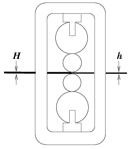
CDS 101/110 Problem set #1, Problem 6. The rolling mill example, hw1rollmill.mdl is a simplified model of a steel rolling mill. The control problem is to control the exit thickness of a sheet of steel that is fed between two rollers.

The exit thickness h of the steel is related to the gap between the rollers, which depends on the unloaded position of backup rollers (also called the screw position), s and the input thickness H. The force on the rollers is reasonably modeled by

F = M ( h - s )

as well as

F = W ( H - h )

where M and W are constants.

Combining these two gives

h ( M + W ) = M s + W H

Measurement and actuator dynamics are modeled with time delays of 1 second and 0.01 seconds, respectively. A proportional-integral control law is incorporated into the model whose job is to try and regulate the output thickness to the desired thickness.

Instructions

Right-click hw1rollmill.mdl and save it to a local drive. Open it with MATLAB (Simulink) and follow the instructions given in Problem Set #1.

Notes:

1. The output thickness for each run is saved to the MATLAB workspace as a structure called "rollmill". You can access the elements of a structure using a period (.), e.g. rollmill.signals...
2. The settling time is the time it takes for the system error to settle to within the desired thickness plus or minus 5%. Any method of finding these values to produce your plots is acceptable, but you may like to investigate the MATLAB "find" command.
3. Include at least ten values in each of your settling time versus Kp/Ki plots.
4. Use the MATLAB "plot" command to produce your plots. Type "help plot" in the MATLAB command window for help on using this function.
5. Include a title, axis labels (with units), and reasonable axis limits on all plots. See MATLAB commands "title", "axis", "ylabel" and "xlabel".